Chi-Square and F-Distributions
Introduction
Up to this point, we’ve looked at probability distributions such as the normal, log-normal, and binomial. These are all useful when we are interested in analyzing the actual values of a variable, such as IQ scores, salaries, or the number of times an event occurs. These distributions describe how individual observations are spread out.
However, there are many situations where we are not focused on individual values themselves, but on the variability within and between distributions. That’s where the chi-square distribution and the F-distribution become important (Wooldridge, 2022).
The chi-square distribution measures how much individual values deviate from their mean. It gives a sense of the total variability within a distribution. The F-distribution, on the other hand, compares the relative variability of two distributions by taking the ratio of their variances. While each distribution on its own might follow a normal shape, the F-distribution tells us whether one set of values is more or less spread out than another.
In short, the chi-square and F distributions allow us to quantify and compare variability, helping us determine whether differences in spread are meaningful or simply due to chance.
When Do We Encounter the Chi-Square Distribution?
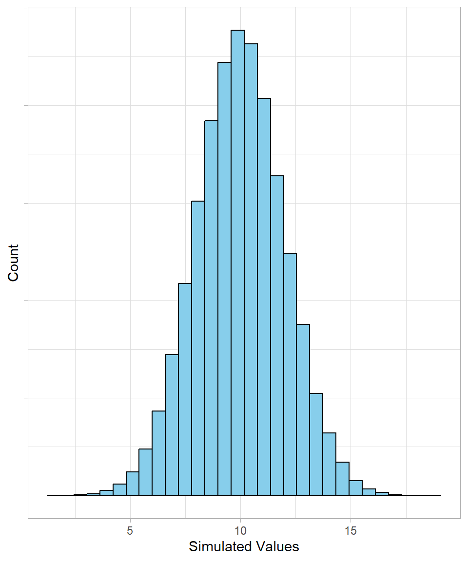
Let’s start with a normal distribution with a mean of 10 and a standard deviation of 2. We can simulate 100,000 values and visualize the results:
Now, we standardize the values (see Chapter Scaling). That means we subtract the mean from each observation and divide by the standard deviation. After this transformation, the distribution looks like this:

Notice that the shape hasn’t changed, but the x-axis values have. The mean is now 0, and most values fall roughly between -3 and +3. Standardization allows us to compare values on the same scale, regardless of the original units.
Next, we square all the standardized values, so that each \(x_i\) becomes \(x^2_i\) . Squaring has two effects: all negative values become positive, and 0 remains the minimum value. The resulting distribution is right-skewed, as shown below:
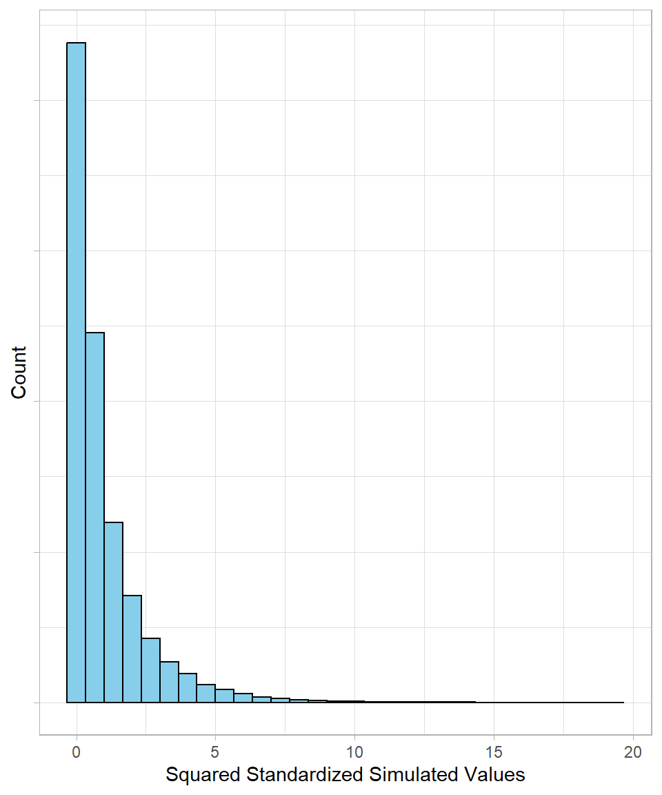
This is the chi-square distribution. What we did here is start with a normal distribution, standardize the values, and square them; this is exactly how a chi-square distribution is generated. Mathematically, we have:
\[\chi^2_i = \left(\frac{x_i - \bar{x}}{\sigma}\right)^2 = Z^2_i\]
The term inside the parentheses is just the z-score, which tells us how far a value is from the mean in standard deviation units. Squaring it emphasizes extreme deviations and ensures all values are positive. Each of these squared values is called a chi-square value, and together they form the chi-square distribution.
There is a direct link between the z-score and the chi-square value: larger absolute z-scores lead to larger chi-square values. Values in the tail of the original normal distribution will appear in the tail of the chi-square distribution as well. Therefore, a chi-square value shows how far a data point is from the mean, measured in squared units of standard deviation.
The key characteristic of the chi-square distribution is what is called the chi-square statistic, which is defined as the sum of all squared standardized deviations. Mathematically, we have:
\[\chi^2 = \sum^n_{i = 1}\left(\frac{x_i - \bar{x}}{\sigma}\right)^2\]
This statistic is very useful because it reflects the total deviation of the observed data from what is expected under the assumed distribution. In other words, it provides a summary measure of how extreme the data are relative to the average spread. The larger the chi-square statistic, the more the observed values collectively deviate from the mean, indicating a greater discrepancy between the data and the expected model.
Because it aggregates all individual squared deviations, the chi-square statistic forms the basis of many statistical tests, something we discuss in more detail in later chapter.
What are the Parameters and Shape of the Chi-Square Distribution?
The chi-square distribution is a continuous distribution defined by a single parameter: its degrees of freedom. The mathematical notation is the following:
\[X \sim \chi^2(df)\]
The reason the degrees of freedom is the only parameter comes from how the variable \(X\) is calculated. Recall that we standardized a normal distribution, which always produces a normal distribution with a mean of 0 and a standard deviation of 1. However, the number of observations we include matters, and this number is captured by the degrees of freedom.
The degrees of freedom reflect the number of squared standardized values that are being summed. With low degrees of freedom, the chi-square distribution is highly right-skewed, with most values clustered near zero and a long tail extending to the right. As the degrees of freedom increase, the distribution becomes less skewed, spreads out more, and gradually approaches the shape of a normal distribution. In other words, the degrees of freedom control how “peaked” or “spread” the distribution is.
The probability density function of the chi-square distribution with \(k\) degrees of freedom is then:
\[f(x) = \frac{1}{2^{\frac{k}{2}}\Gamma(\frac{k}{2})} x^{\frac{k}{2} - 1}e^{(-\frac{x}{2})}\]
This function is defined only for positive values of \(x\) and uses the gamma function (see Chapter Gamma and Exponential Distributions). Thankfully, we do not need to memorize the formula; our goal is to get familiar with its structure. The factor \(x^{k/2-1}\) causes the density to rise from zero, while the exponential term \(e^{(-\frac{x}{2})}\) makes it taper off to the right. The degrees of freedom \(k\) control the shape: small \(k\) gives a peak near zero, and larger \(k\) spreads the distribution and reduces skewness. Looking at the formula this way helps make the chi-square distribution more intuitive, even if we never calculate it by hand.
The expected value a random variable \(X\) that follows a chi-square distribution is just the degrees of freedom:
\[E[X] = df = n - 1\]
This derives mathematically like this:
\[E[X] = E[Z^2_1 + Z^2_2 + ... Z^2_n] = E[Z^2_1] + E[Z^2_2] + ... E[Z^2_n]\]
Plugging in \(Z_{i}^2 = \frac{x_i - \bar{x}}{s}\), we have:
\[E[X] = \left(\frac{x_1 - \bar{x}}{s}\right) ^ 2 + \left(\frac{x_2 - \bar{x}}{s}\right) ^ 2 + ... + \left(\frac{x_n - \bar{x}}{s}\right) ^ 2 =\]
\[\frac{(x_1 - \bar{x})^2 + (x_2 - \bar{x})^2 + ... + (x_n - \bar{x})^2}{s^2} = \frac{\sum_{i = 1}^{n} (x_{i} - \bar{x})^2}{s^2}\]
Since the square power of the standard deviation is \(s^2 = \frac{\sum_{x = 1}^{n} (x_i - \bar{x})^2}{n - 1}\), we have:
\[E[X] = \frac{\sum_{i = 1}^{n} (x_{i} - \bar{x})}{\sum_{i = 1}^{n} (x_{i} - \bar{x})} \cdot (n-1) = n - 1\]
Deriving the variance is a more complicated task, but mathematically we have:
\[Var[X] = Var[Z^2_1 + Z^2_2 + ... Z^2_n] = Var\left(\left(\frac{x_1 - \bar{x}}{s}\right) ^ 2 + \left(\frac{x_2 - \bar{x}}{s}\right) ^ 2 + ... + \left(\frac{x_n - \bar{x}}{s}\right) ^ 2 \right) = 2k\]
Even though we could show in more detail complicated formula, the conclusion will remain the same: the variance is simply two times the degrees of freedom.
When Do We Encounter the F Distribution?
Previously, the focus was on the variability of a single distribution. We now shift our attention to the comparison of variability between two distributions. Recall that a chi-square distribution is formed from a chi-square statistic, defined as the sum of squared deviations from the original mean. The F-distribution arises from combining two such chi-square statistics through a ratio. In essence, the collection of possible ratios formed from the chi-square statistics of two independent chi-square distributions generates the F-distribution.
\[F\text{-distribution} \;=\; \frac{\text{Chi-Square}_1}{\text{Chi-Square}_2}\]
The purpose of this distribution is therefore to compare the variability of two distributions. Just as a chi-square distribution is associated with individual chi-square values (or squared z-scores), the F-distribution is associated with its own F-values and an F-statistic. An F-value represents an individual observation from the F-distribution, while the F-statistic is defined as the ratio of two scaled chi-square statistics:
\[F = \frac{\chi^2_1/df_1}{\chi^2_2/df_2}\]
Looking at this formula, we realize the following: each chi-square statistic is normalized (divided) by its own degrees of freedom, something that leads to the average squared deviation. This is actually the same concept as the variance, meaning we can write the formula above like this:
\[F = \frac{\chi^2_1/df_1}{\chi^2_2/df_2} = \frac{\sigma^2_1}{\sigma^2_2}\]
If the two distributions exhibit similar variability, their corresponding variances will be approximately equal, and their ratio will therefore be close to 1. In contrast, if one distribution displays substantially greater variability than the other, the resulting F-statistic will deviate significantly from 1, becoming either much larger or much smaller depending on which distribution has greater spread.
An example of an F-distribution is shown in the plot below:
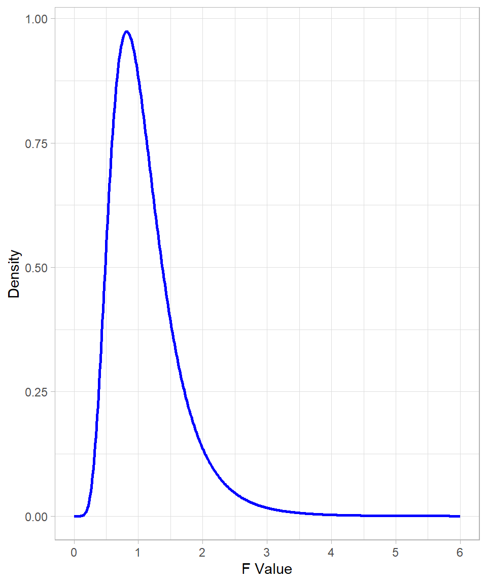
The expected value (mean) of this distribution is approximately 1. This value does not lie at the peak of the distribution, since it is pulled to the right by the extreme values in the long right tail. It is also clear that the value 0 has zero density (zero likelihood), which is intuitive: a chi-square statistic cannot be 0, because this would imply zero variability, and without variability a distribution cannot exist.
What are the Parameters and Shape of the F Distribution?
The F-distribution is a continuous probability distribution that arises when comparing two variances. To note that a random variable \(X\) follows an F-Distribution, we write:
\[X \sim F(df_1, df_2)\]
where:
\(df_1\) is the degrees of freedom from the numerator sample
\(df_2\) is the degrees of freedom from the denominator sample
These parameters should be expected; since the F-distribution is defined as the ratio of two chi-square distributions and the only parameter of each distribution is its degrees of freedom, the F-distribution has both degrees of freedom as its own parameters. These parameters define the shape of the F-distribution, whose shape is also right skewed.
Just like the chi-square distribution, the F-distribution has a probability density function with degrees of freedom \(df_1\) and \(df_2\), and is given by:
\[f(x) = \frac{1}{B\left(\frac{d_1}{2}, \frac{d_2}{2}\right)} \left( \frac{d_1}{d_2} \right)^{d_1/2} \times \frac{x^{(d_1/2 - 1)}}{\left(1 + \frac{d_1}{d_2}x\right)^{(d_1 + d_2)/2}}, \quad x > 0\]
There’s no need to memorize this formula. What’s important is to understand the role of the F-distribution: it is simply the ratio of two chi-square distributions.
The expected value tells us where the center of the F-distribution lies. It only exists when the denominator \(df_{2}\) is greater than 2 and is given by the following formula:
\[E[X] = \frac{df_2}{df_2 - 2}\]
The \(-2\) in the denominator derives from the beta function in the probability density function, making it important because it reflects how the F-distribution behaves near zero. At this point, there is no need to go into more mathematical details, as our goal is to understand the expected value of the F-distribution, which highlights something important: it depends only on the degrees of freedom of the chi-square distribution in the denominator.
The reason it’s only the denominator that matters is intuitive: the denominator determines the stability of the ratio. A very small denominator can make the F-statistic extremely large, while the numerator only scales the ratio. That’s why the expected value formula only depends on \(df_2\).
Technically, we could choose whether the larger chi-square statistic goes to the numerator or denominator of the ratio, but usually we prefer to place it in the numerator. The reason is mostly about interpretability: putting the larger variance in the numerator makes the F-statistic easier to read. Values above 1 naturally indicate that the first distribution has more variability than the second, while values near 1 indicate similar variances. If the larger variance were in the denominator, the ratio would often be less than 1, which is less convenient for interpretation.
Regarding the variance, since the F-distribution is a ratio of sample variances, its own variance reflects how much the two sample variances differ relative to each other.
As the degrees of freedom increase, the distribution becomes more concentrated:
\[Var[X] = \frac{2 \cdot df_2^2 \cdot (df_1 + df_2 - 2)}{df_1 \cdot (df_2 - 2)^2 \cdot (df_2 - 4)}, \quad \text{for } df_2 > 4\]
We don’t need to go into the full mathematical details. The key points are that the denominator’s degrees of freedom must be greater than 4 for the variance to exist, and that the variance depends on the degrees of freedom of both distributions.
Calculating and Simulating in R
Base R provides built-in functions to work with both the chi-square and F distributions. These allow us to simulate values, calculate probabilities, and visualize shapes, just as we did with other distributions.
Let’s simulate this idea directly. The rchisq() function generates random values from a chi-square distribution with a given number of degrees of freedom. For example, if we simulate the sum of 2 squared standard normal values, that’s a chi-square with 2 degrees of freedom:
# Setting seed
set.seed(111)

# Simulating 10,000 chi-square values with 2 degrees of freedom
chi_values <- rchisq(n = 10000, df = 2)

# Printing the first 10 values
head(chi_values, n = 10)
[1] 1.3603167 0.5869620 0.7297102 0.7729441 1.3486507 7.3308092 0.7694690
[8] 0.6340439 1.6349160 2.4459015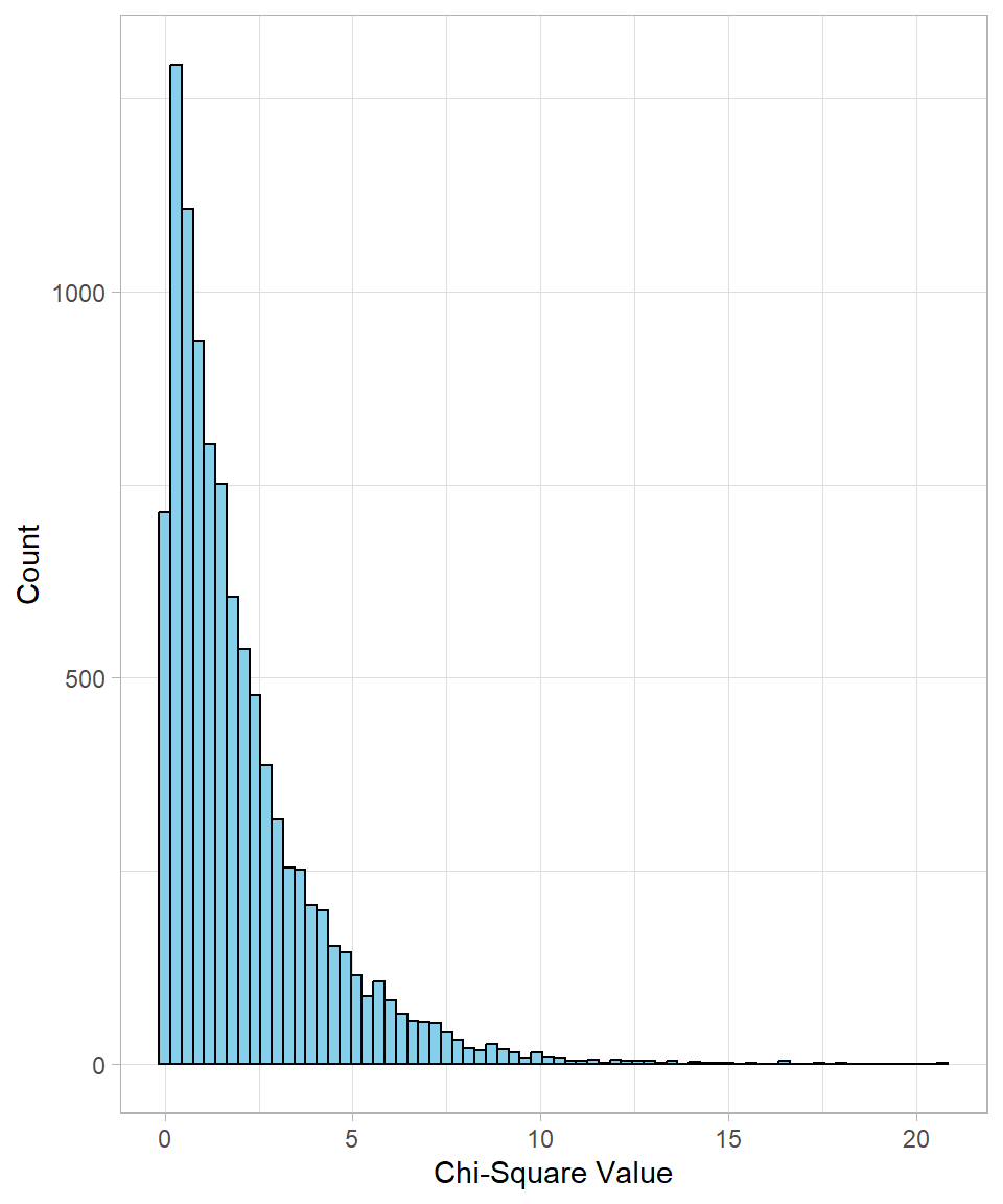
The distribution is skewed to the right, as expected. With more degrees of freedom, the distribution becomes more symmetric.
To calculate the exact probability density at a point, say x = 3, we use the dchisq() function:
# Density at x = 3 for df = 2
dchisq(x = 3, df = 2)
[1] 0.1115651The probability that a chi-square value is less than or equal to 3 can be calculated using the function pchisq():
# Cumulative probability up to 3
pchisq(q = 3, df = 2)
[1] 0.7768698Lastly, to find the value that marks the 90th percentile (i.e., the value below which 90% of the values fall), we can apply the function qchisq():
# 90th percentile of chi-square with df = 2
qchisq(p = 0.9, df = 2)
[1] 4.60517Just like the chi-square distribution, the F-distribution is skewed to the right, especially when the degrees of freedom are small. Using the function rf(), we can simulate F values by specifying the degrees of freedom for the two distributions of interest:
# Setting seed
set.seed(111)

# Simulating 10,000 f values with 5 and 10 degrees of freedom
f_values <- rf(n = 10000, df1 = 5, df2 = 10)

# Printing the first 10 values
head(f_values, n = 10)
[1] 1.2266795 0.8295111 2.8212198 0.3439007 0.2760569 0.8175617 0.1834832
[8] 0.2052966 0.5787551 0.5558969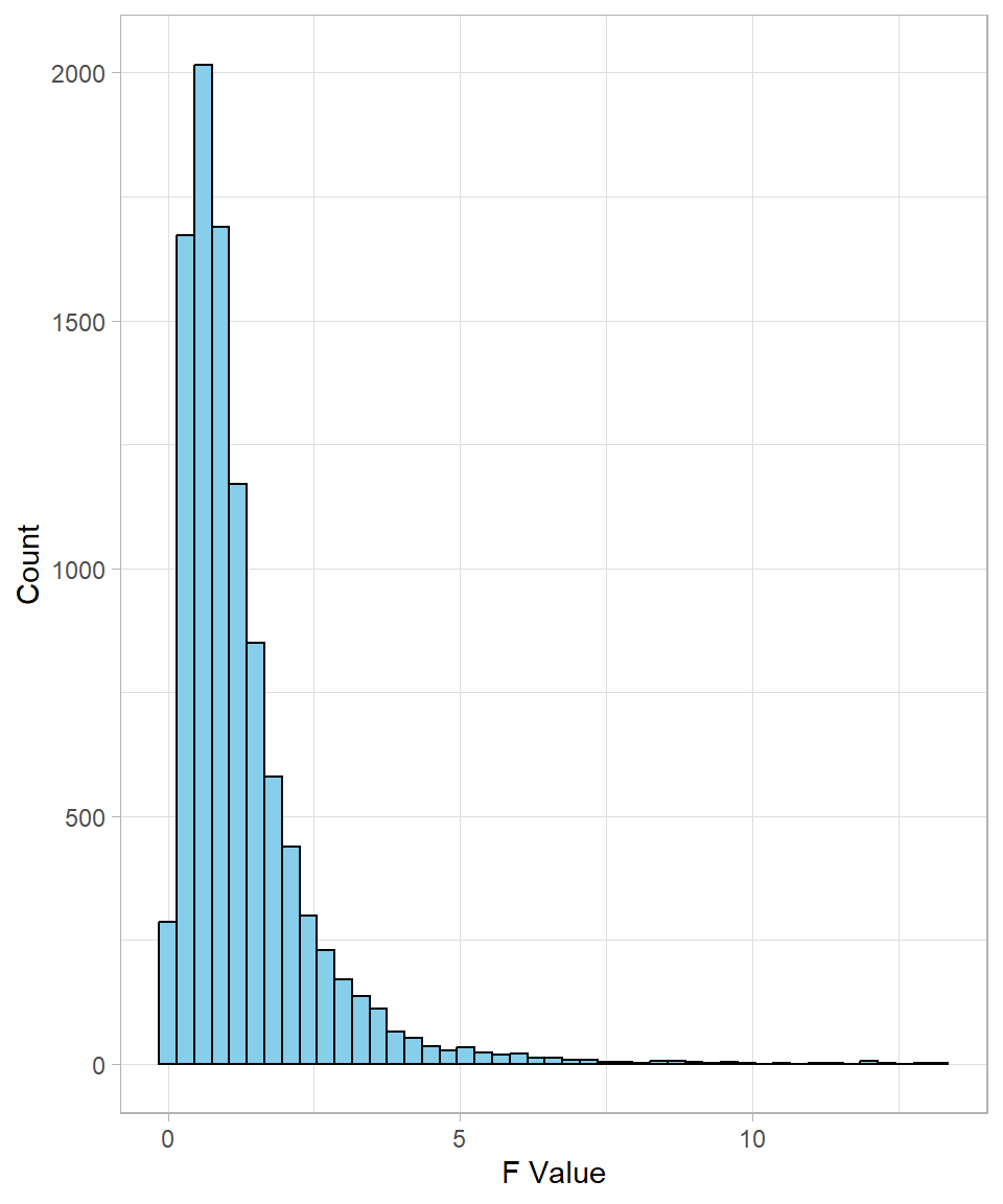
To find the value of the probability density function (the height of the curve) at a specific point, we use the function df():
# Density of F at x = 2
df(x = 2, df1 = 5, df2 = 10)
[1] 0.1620057For calculating the cumulative probability (i.e., the probability that the F-statistic is less than or equal to a certain value), the function pf() is applied:
# Cumulative probability of F ≤ 2
pf(q = 2, df1 = 5, df2 = 10)
[1] 0.835805Finally, to find the 95th percentile (a typical threshold for larger values), we use the function qf():
# 95th percentile of F-distribution
qf(p = 0.95, df1 = 5, df2 = 10)
[1] 3.325835Recap
The chi-square distribution measures the total squared deviations from expected values, while the F-distribution compares two variances by taking the ratio of two independent chi-square variables, each divided by its respective degrees of freedom.
The key takeaway is that these distributions provide tools for quantifying variability and comparing differences in a meaningful way. Both form an essential foundation for understanding statistical tests, which we explore in more detail in the next chapters.